hugging face基础入门——evaluate库的使用

hugging face基础入门——evaluate库的使用

引用

CSDN

1.

https://blog.csdn.net/weixin_56696781/article/details/144017236

内容前置

本系列下内容为跟随b站课程总结 课程链接：
【手把手带你实战HuggingFace Transformers】
本节内容主要是evaluate库的一些操作并修改之前编写的部分评估代码。

evaluate库的使用

首先我们可以通过下面方法查看evaluate支持的评估函数：

import evaluate
evaluate.list_evaluation_modules()  

输出结果为

['Remeris/rouge_ru',
 'hage2000/code_eval_stdio',
 'lvwerra/test',
 'jordyvl/ece',
 'angelina-wang/directional_bias_amplification',
 'cpllab/syntaxgym',
 'lvwerra/bary_score',
 'hack/test_metric',
 'yzha/ctc_eval',
 'codeparrot/apps_metric',
 'mfumanelli/geometric_mean',
 'daiyizheng/valid',
 'erntkn/dice_coefficient',
 'mgfrantz/roc_auc_macro',
 'Vlasta/pr_auc',
 'gorkaartola/metric_for_tp_fp_samples',
 'idsedykh/metric',
 'idsedykh/codebleu2',
 'idsedykh/codebleu',
 'idsedykh/megaglue',
 'christopher/ndcg',
 'Vertaix/vendiscore',
 'GMFTBY/dailydialogevaluate',
 'GMFTBY/dailydialog_evaluate',
 'jzm-mailchimp/joshs_second_test_metric',
...
 'lsy641/distinct',
 'grepLeigh/perplexity',
 'Charles95/element_count',
 'Charles95/accuracy',
 'Lucky28/honest']  

这里我们加载下常用的accuracy看下

acc = evaluate.load("accuracy")
acc  

输出结果为

EvaluationModule(name: "accuracy", module_type: "metric", features: {'predictions': Value(dtype='int32', id=None), 'references': Value(dtype='int32', id=None)}, usage: """
Args:
    predictions (`list` of `int`): Predicted labels.
    references (`list` of `int`): Ground truth labels.
    normalize (`boolean`): If set to False, returns the number of correctly classified samples. Otherwise, returns the fraction of correctly classified samples. Defaults to True.
    sample_weight (`list` of `float`): Sample weights Defaults to None.
Returns:
    accuracy (`float` or `int`): Accuracy score. Minimum possible value is 0. Maximum possible value is 1.0, or the number of examples input, if `normalize` is set to `True`.. A higher score means higher accuracy.
Examples:
    Example 1-A simple example
        >>> accuracy_metric = evaluate.load("accuracy")
        >>> results = accuracy_metric.compute(references=[0, 1, 2, 0, 1, 2], predictions=[0, 1, 1, 2, 1, 0])
        >>> print(results)
        {'accuracy': 0.5}
    Example 2-The same as Example 1, except with `normalize` set to `False`.
        >>> accuracy_metric = evaluate.load("accuracy")
        >>> results = accuracy_metric.compute(references=[0, 1, 2, 0, 1, 2], predictions=[0, 1, 1, 2, 1, 0], normalize=False)
        >>> print(results)
        {'accuracy': 3.0}
    Example 3-The same as Example 1, except with `sample_weight` set.
        >>> accuracy_metric = evaluate.load("accuracy")
        >>> results = accuracy_metric.compute(references=[0, 1, 2, 0, 1, 2], predictions=[0, 1, 1, 2, 1, 0], sample_weight=[0.5, 2, 0.7, 0.5, 9, 0.4])
        >>> print(results)
        {'accuracy': 0.8778625954198473}
""", stored examples: 0)  

我们可以看到里面提供了具体参数及样例使用从而帮助我们理解。

但我们数据往往是逐步按批次处理的，那么我们就得奖代码改写为：

#流式数据处理
for pred,truth in zip([1,1,1,0,1],[1,0,1,1,1]):
    acc.add(prediction=pred,reference=truth)
acc.compute()
#输出为{'accuracy': 0.6}
#批次数据处理
for batch_pre,batch_tru in [[[1,1,0],[1,0,0]],[[1,1,1],[0,1,0]]]:
    print(batch_pre)
    print(batch_tru)
    acc.add_batch(predictions=batch_pre,references=batch_tru)
acc.compute()
#输出为[1, 1, 0]
#      [1, 0, 0]
#      [1, 1, 1]
#      [0, 1, 0]
#{'accuracy': 0.5}  

第一种方法（
acc.add(prediction=..., reference=...)
）更适合实时处理数据，逐步计算每个预测值和真实值的准确率。它可以在训练的每一个小批次中逐步更新结果。

第二种方法（
acc.add_batch(predictions=..., references=...)
）则更适合一次性处理一个批次的数据，通常在训练模型时会使用批量数据，因此这种方式更加高效，尤其是在计算多个样本的准确率时。

当我们需要使用多种评估函数时我们使用自带的combine函数：

combines = evaluate.combine(["accuracy","f1","recall","precision"])
combines_result_1 = combines.compute(predictions=[1,1,0,0],references=[1,0,1,0])
combines_result_1  

输出为：

{'accuracy': 0.5, 'f1': 0.5, 'recall': 0.5, 'precision': 0.5}  

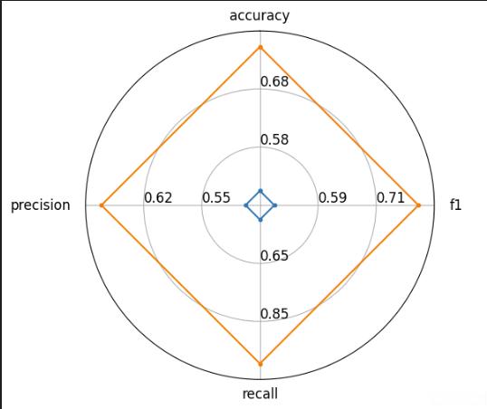
为了更好理解模型之前性能区别，evaluate还提供了radar_plot函数为我们绘制雷达图，这里我随意据两个案例说明：

combines_result_1 = combines.compute(predictions=[1,1,0,0],references=[1,0,1,0])
#输出为{'accuracy': 0.5, 'f1': 0.5, 'recall': 0.5, 'precision': 0.5}
combines_result_2 = combines.compute(predictions=[1,1,1,0],references=[1,0,1,0])
#输出为{'accuracy': 0.75, 'f1': 0.8, 'recall': 1.0, 'precision': 0.6666666666666666}
from evaluate.visualization import radar_plot
data = [
    combines_result_1,
    combines_result_2
]
model_names = ["model1","model2"]
plot = radar_plot(data,model_names=model_names)  

输出雷达图为：

原函数修改

学习了evaluate库之后，我们可以对hingingface基础入门——小模型全量微调-CSDN博客中评估函数进行修改并增加，原函数为：

def eval():
    model.eval()
    acc = 0
    with torch.no_grad():  # 推理模式
        for batch in validloader:
![](https://wy-static.wenxiaobai.com/chat-rag-image/18008102769810952882)
            if torch.cuda.is_available():
                batch = {k: v.cuda() for k, v in batch.items()}
            output = model(**batch)
            pred = torch.argmax(output.logits, dim=-1)
            acc += (pred == batch["labels"]).float().sum().item()  # 累计正确预测数
    return acc / len(validset)  

修改后函数为：

combines = evaluate.combine(["accuracy","f1"])
def eval():
    model.eval()
    acc = 0
    with torch.no_grad():  # 推理模式
        for batch in validloader:
            if torch.cuda.is_available():
                batch = {k: v.cuda() for k, v in batch.items()}
            output = model(**batch)
            pred = torch.argmax(output.logits, dim=-1)
            combines.add(prediction==pred,reference=bath["labels"])
            return combines.compute()  

如有讲解不周到之初，欢迎指出交流，请大家多多包涵