数据科学中的 R 语言

数据科学中的 R 语言

第 63 章 机器学习

Rstudio工厂的Max Kuhn大神正主持机器学习的开发，日臻成熟了，感觉很强大啊。

63.2 机器学习

split <- penguins %>% 
  mutate(species = fct_lump(species, 1)) %>% 
  initial_split()
split
training_data <- training(split)
training_data
testing_data <- testing(split)
testing_data  

63.7 workflow

63.7.1 使用 recipes

参考tidy modeling in R, 被预测变量在分割前，应该先处理，比如标准化。 但这里的案例，我为了偷懒，被预测变量
bill_length_mm
，暂时保留不变。 预测变量做标准处理。

penguins_lm <- 
  #parsnip::set_engine("lm") 
penguins_recipe  <- 
  recipes::recipe(bill_length_mm ~ bill_depth_mm + sex, data = training_data) %>% 
  recipes::step_normalize(all_numeric(), -all_outcomes()) %>% 
  recipes::step_dummy(all_nominal())
broom::tidy(penguins_recipe)  

  
## # A tibble: 2 × 6
##   number operation type      trained skip  id             
##    <int> <chr>     <chr>     <lgl>   <lgl> <chr>          
## 1      1 step      normalize FALSE   FALSE normalize_zs0oP
## 2      2 step      dummy     FALSE   FALSE dummy_Rh8f7  

63.7.2 workflows的思路更清晰

workflows的思路让模型结构更清晰。 这样
prep()
,
bake()
, and
juice()
就可以省略了，只需要recipe和model，他们往往是成对出现的

wflow <- 
  workflows::add_recipe(penguins_recipe) %>% 
  workflows::add_model(penguins_lm) 
wflow_fit <- 
  wflow %>% 
  parsnip::fit(data = training_data)  

wflow_fit %>% 

## # A tibble: 3 × 3
##   term          estimate std.error
##   <chr>            <dbl>     <dbl>
## 1 (Intercept)      41.1      0.442
## 2 bill_depth_mm    -2.33     0.297
## 3 sex_male          5.68     0.634  

wflow_fit %>% 

先提取模型，用在
predict()
是可以的，但这样太麻烦了

wflow_fit %>% 
  stats::predict(new_data = test_data) # note: test_data not testing_data  

因为，
predict()
会自动的将recipes(对training_data的操作)，应用到testing_data 这个不错，参考这里

penguins_pred <- 
  predict(
    wflow_fit, 
    new_data = testing_data %>% dplyr::select(-bill_length_mm), # note: testing_data not test_data
    type = "numeric"
  ) %>% 
  dplyr::bind_cols(testing_data %>% dplyr::select(bill_length_mm))
penguins_pred  

## # A tibble: 84 × 2
##    .pred bill_length_mm
##    <dbl>          <dbl>
##  1  40.2           38.9
##  2  42.5           42.5
##  3  45.6           37.2
##  4  41.2           36.4
##  5  43.3           38.8
##  6  39.4           42.2
##  7  44.4           39.8
##  8  40.0           36.5
##  9  39.4           36  
## 10  43.7           44.1
## # ℹ 74 more rows  

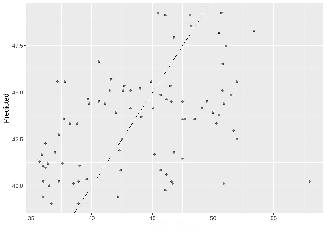
penguins_pred %>% 
  ggplot(aes(x = bill_length_mm, y = .pred)) + 
  labs(y = "Predicted ", x = "bill_length_mm")   

augment()
具有
predict()
一样的功能和特性，还更简练的多

wflow_fit %>%
  augment(new_data = testing_data) %>%       # note: testing_data not test_data
  ggplot(aes(x = bill_length_mm, y = .pred)) + 
  labs(y = "Predicted ", x = "bill_length_mm")   

63.7.3 模型评估

参考https://www.tmwr.org/performance.html#regression-metrics

penguins_pred %>%
  yardstick::rmse(truth = bill_length_mm, estimate = .pred)   

## # A tibble: 1 × 3
##   .metric .estimator .estimate
##   <chr>   <chr>          <dbl>
## 1 rmse    standard        4.94  
![](https://wy-static.wenxiaobai.com/chat-rag-image/1842725041372192560)

自定义一个指标评价函数my_multi_metric，就是放一起，感觉不够tidyverse

my_multi_metric <- yardstick::metric_set(rmse, rsq, mae, ccc)
penguins_pred %>%
  my_multi_metric(truth = bill_length_mm, estimate = .pred)   

## # A tibble: 4 × 3
##   .metric .estimator .estimate
##   <chr>   <chr>          <dbl>
## 1 rmse    standard       4.94 
![](https://wy-static.wenxiaobai.com/chat-rag-image/7978151746396179886)
## 2 rsq     standard       0.179
## 3 mae     standard       4.10 
## 4 ccc     standard       0.335